Always-on and low-variance channels
Three client questions arrive together when a channel runs at a near-constant level. “Why does the model give search almost no credit?” “Why can’t you model our affiliate channel?” “Can you tighten the prior so the affiliate interval is usable?”
The answer to the third is no, and this note exists to make that refusal defensible. An additive MMM estimates a channel’s effect from the contrast between periods of high and low transformed exposure. A channel that never moves supplies no contrast. Its coefficient is then set by the prior and the functional form, and the fit reports that number with an interval as if the data had produced it. Tightening the prior narrows the interval without adding information about the channel, and it removes the one signal, the width, that told the reader the data were silent.
The first two questions often share this root. Search frequently has a second problem that presents the same symptom, and the note separates the two.
The FE and CRE pages own the estimability gate and its threshold table. This note owns the case the gate does not catch: a channel with enough variation to pass and too little to inform.
Three regimes, not two
Analysts tend to treat identification as binary. Either the design is degenerate and the fit fails, or it is not and the coefficient is usable. AMMM3’s behaviour has three regimes, and the middle one is where always-on channels live.
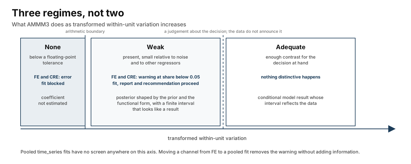
| Regime | Transformed within-unit variation | What AMMM3 does | What the coefficient is |
|---|---|---|---|
| None | Within-unit sum of squares below a floating-point tolerance | FE and CRE raise an error before the graph is built. Pooled time_series fits do not check. | Not estimated |
| Weak | Present, small relative to noise and to other regressors | FE and CRE warn when the within-variation share is below 0.05. The fit, the report and any budget recommendation proceed. Pooled fits do not check. | A posterior shaped by the prior and the functional form, with a finite interval |
| Adequate | Enough contrast for the decision at hand | Nothing distinctive | A conditional model result whose interval reflects the data |
The boundary between the first two regimes is arithmetic. The boundary between the second and third is a judgement about the decision, and the data do not announce it. Ask how narrow the interval on this channel’s contribution or marginal return must be before the client would act differently at one end of it than at the other. A channel whose 94% interval on ROAS runs from 0.5 to 8 is in the weak regime for a budget reallocation and may be in the adequate regime for a decision to keep it running at all. Record the tolerance before fitting, as the Agency Workflow requires, and classify the channel against it afterwards.
The zero-variation gate is numerical
The FE screen flags a predictor when its within-unit sum of squares, computed
on transformed media at the reference point, falls below the square of a
tolerance built from floating-point epsilon, the largest absolute transformed
value and the square root of the number of cells. The implementation in
src/abacus/mmm/models/fixed_effects_estimability.py describes it as “a
numerical, rather than substantive, zero-variation tolerance”. It catches a
design that is degenerate in arithmetic. It cannot catch a design that is
degenerate for the decision, because that depends on the noise level, the
other regressors and the tolerance the client has for being wrong.
A warning obliges the analyst, and blocks nothing
FE and CRE do have a weak-variation diagnostic. within_variation_share_warning
defaults to 0.05 in both FixedEffectsEstimabilityConfig and
CREEstimabilityConfig, alongside VIF above 20 and condition number at least
30. All three are warnings. The pipeline continues, the report is written to
10_pre_diagnostics/fixed_effects_estimability.csv and .json, and no later
stage refuses to run because of it.
A warning therefore places an obligation on the analyst rather than on the software. Open the report. Record the flagged variable’s within-variation share and VIF. State whether the decision at stake survives a coefficient that the data barely inform. Write that judgement into the deliverable. A warning that is read and not acted on has the same effect as no warning.
Two further limits follow from how the screen is built. It evaluates the configured adstock and saturation at a fixed-seed PyMC initial point, so it is a reference-design diagnostic and not a proof of identification across the posterior. And the share is a within-to-total ratio. A channel can hold a share above 0.05 with a within-unit spread that is still far too small for the decision.
Pooled fits have no screen
The estimability reports belong to FE, CRE and the categorical FE time
surface. A PanelMMM fitted as one aggregate time_series with an always-on
channel receives no zero-variation error, no share warning and no VIF warning.
The estimators with the strictest identification requirements are also the
only ones that tell you about it. Moving an unestimable channel from an FE
panel to a pooled national fit removes the warning without adding information.
What a weakly identified coefficient is reporting
PanelMMM builds an additive mean on the scaled target,
where
is the mean of the scaled target in week
,
is the
intercept,
is channel
’s max-abs scaled spend after adstock,
is LogisticSaturation with curvature
,
is the
channel amplitude, and
is the vector of controls with coefficients
. The likelihood learns about
from the spread of
its regressor around its own mean, because the intercept absorbs the mean.
Holding the transform parameters fixed,
where is the residual standard deviation on the scaled target, is the number of observations, is the mean of the transformed regressor and is its design spread, the standard deviation of the transformed channel around its own mean.
As the likelihood becomes flat in . It also becomes flat in and in the adstock decay , because a channel held at one operating point traces no part of its response curve and produces no carryover contrast. The posterior in those directions is the prior:
up to whatever the intercept prior contributes through the trade-off .
The consequence for each reported quantity is concrete. The contribution in
target units is
, where
is the
target scale from mmm.data.get_target_scale(). Under the default
HalfNormal(2) prior,
, and an
always-on channel scaled to
with
at its prior
mean of 3 has
. The prior alone therefore implies a mean
weekly contribution of about
, more than the whole scaled target,
and only the intercept prior and whatever weak information remains pull it
down. Divide by spend and the result is a finite ROAS. Trace
across a spend range and the result is a response curve with a plateau at
and a half-saturation point at
on the scaled
axis, with intervals on both.
None of this is random and none of it comes from the data on this channel. It is the prior, propagated through the transform, and it will look like a result. See Bayesian priors for econometricians for the general point that a posterior can resemble its prior for three different reasons.
Why the transforms shrink variation further
The FE page notes that adstock can change the screen’s result. The mechanism matters because it decides which kinds of raw variation survive to the design matrix, and an always-on channel usually has the kind that does not.
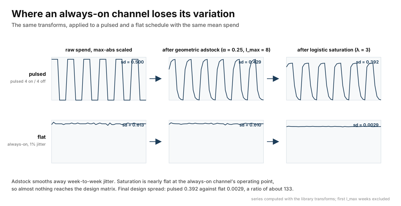
The figure applies the reference transforms to two schedules with the same mean spend. The pulsed channel’s design spread survives both steps. The flat channel loses variation twice, once to smoothing and once to compression, and the two losses multiply. The mechanisms follow.
Adstock is a low-pass filter
GeometricAdstock with normalize=True applies non-negative weights that sum
to one across l_max lags,
where
is raw spend in week
,
is its adstocked value,
is the decay parameter,
is l_max and
is the
normalised weight on the spend
weeks back.
A constant passes through unchanged. A slow drift passes through almost unchanged. Week-to-week jitter with variance comes out with variance , which is below whenever . At and , , so the jitter’s standard deviation is multiplied by . At it is multiplied by . An always-on channel’s variation is mostly jitter, so adstock removes most of what it has and keeps the slow movements it does not have.
Saturation compresses variation where the curve is flat
The derivative of the logistic saturation is
A channel held near an operating point contributes transformed variation of about times its adstocked variation. At , , and . The compression is severe at both ends: near zero because is near zero, and near the plateau because has stopped rising.
Max-abs scaling puts an always-on channel at the plateau end. Its maximum is
close to its mean, so its scaled operating point is close to one, and under
the default Gamma(3, 1) prior on
the reference design places it
where
is smallest. The channel’s raw variance is irrelevant to this; the
operating point decides it.
The two effects multiply
A channel invoiced at about 50 a week with 1% jitter has a scaled standard deviation of about . After adstock at that is . After saturation at and it is . A channel pulsed between zero and its maximum has a scaled standard deviation of and a transformed standard deviation of about , because it spends its time where the curve is steep and crosses the whole of it. The ratio of design spreads is about 150, and the ratio of Fisher information is its square. A channel can show visible movement on a spend chart and still supply almost nothing to the design matrix. The worked example computes both numbers.
Zero-padded history creates a false contrast
AMMM3 pads pre-sample adstock history with zeros. Every channel’s transformed
series therefore ramps up over its first l_max weeks. For a channel with
real contrasts this is negligible. For an always-on channel that was running
before the data start, it is the largest source of transformed variation in
the sample, and it is an artefact: the true carryover was already at steady
state in week one. The model has two ways to reconcile the ramp in its
regressor with the absence of a ramp in the outcome. It can shrink
,
or it can shrink
so that the ramp disappears. Either way the
coefficient is being shaped by the boundary of the data and not by the
channel. Compute the transformed screen with and without the first l_max
weeks. If the two differ materially, the boundary is doing the identifying.
Screens to run before fitting
Run these on every channel before the first fit and record the results with the model specification. Each rules out one failure and none of them establishes identification.
Transformed within-unit variation at the reference point. For FE and CRE, read
within_variation_sharefrom the estimability report. For a pooled fit, compute the standard deviation of the transformed channel yourself at the prior means of the transform parameters, as the worked example does. This rules out a design that is flat at the reference point. It does not rule out weak identification at other parameter values, because the transform parameters are estimated.Coefficient of variation of raw spend. This rules out a channel whose level never moves. A CV below a few percent is a flag regardless of the transform, because no transform manufactures contrast.
Number of distinct spend levels and the length of the longest constant run. This rules out retainer-style spend. A channel with three levels is identified from at most two contrasts. A constant run of twenty weeks is twenty observations that inform the intercept and not the channel.
Collinearity of the transformed channel with the other transformed channels, with a linear trend and with the seasonal basis. An always-on channel is frequently near-collinear with the intercept, because a constant is the intercept, and with a trend, because its only movement is a slow drift. For a pooled fit the transformed standard deviation from screen 1 is the collinearity with the intercept. For FE and CRE read the VIF and condition number from the report.
Prior sensitivity. Refit under at least one alternative prior on
saturation_betaand one onsaturation_lam, and compare the channel’s contribution and marginal return. A posterior that moves with the prior is the direct evidence that the data are not identifying the coefficient. The runner plans these fits through the prior-sensitivity API; scenario expansion writes the configurations and does not run them.
If you want a number for screen 1, derive it from the decision. For a 94% interval on with half-width , the design spread must satisfy
With scaled residual noise , and , this gives . That is a floor, because it assumes and are known and no other regressor competes for the same variation. Halve and the floor doubles. Add a flexible baseline and it rises further. Report the reasoning with the number.
Worked example: pulsed against flat
Two weekly datasets share the same TV spend, the same noise draws, the same
true response curve for an affiliate channel in raw spend units and nearly the
same total affiliate spend over three years, 8000 against 7810. In the first,
affiliate runs four weeks on at 100 and four weeks off. In the second, it
invoices about 50 every week, rounded to whole units, with a coefficient of
variation near 1%. Both channels have been running for l_max weeks before
the first retained date, so the sample starts at steady state as real
always-on data do. The fitted model does not see that history.
Each dataset is fitted three times with the same specification and three
priors on the affiliate amplitude: the default HalfNormal(2), a tightened
HalfNormal(0.5) that answers the client’s literal request, and an
informative Gamma(mu=0.3, sigma=0.03) centred above the true flat
contribution, so that the example can show whether the data correct it.
What to expect
The screen should show the pulsed affiliate with a transformed standard
deviation near
and the flat affiliate near
once the first
l_max weeks are excluded, with a larger whole-sample figure caused by the
zero-padding ramp.
For the pulsed channel, with on the scaled target, and gives about . The contribution should be recovered within a few percent if were known, wider in practice because and are estimated jointly, and it should not move across the three priors.
For the flat channel the same formula with
gives about
,
which is the standard deviation of the HalfNormal(2) prior. The default
posterior should therefore be a compromise between a nearly flat likelihood
and the prior, with a mean well above the true value and an interval spanning
several times it. The tightened prior should narrow the interval by roughly
the ratio of prior scales, and the informative prior should return itself.
should match its prior in all three flat fits. The contribution
interval should stay wide under the informative prior, because
remains free.
The fit
import arviz as az
import numpy as np
import pandas as pd
from pymc_extras.prior import Prior

from abacus.mmm import GeometricAdstock, LogisticSaturation
from abacus.mmm.panel import PanelMMM
from abacus.mmm.transforms import geometric_adstock, logistic_saturation

L_MAX = 8
TRUE_ALPHA = 0.3
TRUE_AMPLITUDE = 2000.0  # weekly revenue at full saturation, both datasets
TRUE_HALF_SATURATION = 40.0  # raw spend units, both datasets
# Prior means of the default Beta(1, 3) decay and Gamma(3, 1) curvature priors.
# The fixed-seed PyMC initial point used by the FE screen takes the same values.
REFERENCE_ALPHA = 0.25
REFERENCE_LAM = 3.0
BETA_PRIORS = {
    "default HalfNormal(2)": Prior("HalfNormal", sigma=2.0),
    "tightened HalfNormal(0.5)": Prior("HalfNormal", sigma=0.5),
    "informative Gamma(mu=0.3, sigma=0.03)": Prior("Gamma", mu=0.3, sigma=0.03),
}


def transformed(spend: np.ndarray, alpha: float, lam: float) -> np.ndarray:
    """Return spend after normalised geometric adstock and logistic saturation.

    The library transform functions are used so that the screen and the
    generating process apply the same operations as the fitted model,
    including zero padding of the history before the first observation.
    """
    carried = geometric_adstock(spend, alpha=alpha, l_max=L_MAX, normalize=True)
    return np.asarray(logistic_saturation(carried, lam=lam).eval(), dtype=float)


def make_datasets(seed: int = 3, n_weeks: int = 156) -> dict[str, pd.DataFrame]:
    """Return two weekly datasets that differ only in how affiliate is scheduled.

    Both share the same TV spend, the same noise draws, the same true affiliate
    response curve in raw spend units and nearly the same total affiliate spend.
    The pulsed dataset alternates four weeks on at 100 with four weeks off. The flat
    dataset invoices about 50 every week, rounded to whole units. Spend runs for
    ``L_MAX`` weeks before the first retained date, so the retained sample
    starts at steady state, as an always-on channel does in real data. The
    fitted model does not see that history and pads it with zeros.
    """
    rng = np.random.default_rng(seed)
    total = n_weeks + L_MAX
    dates = pd.date_range("2022-01-03", periods=n_weeks, freq="W-MON")
    tv = rng.gamma(shape=2.0, scale=40.0, size=total)
    jitter = rng.normal(scale=0.6, size=total)
    noise = rng.normal(scale=300.0, size=total)
    schedules = {
        "pulsed": 100.0 * (np.arange(total) // 4 % 2 == 0),
        "flat": np.round(50.0 + jitter),
    }
    tv_effect = 1500.0 * transformed(tv, TRUE_ALPHA, np.log(3.0) / 60.0)
    datasets = {}
    for name, affiliate in schedules.items():
        affiliate_effect = TRUE_AMPLITUDE * transformed(
            affiliate, TRUE_ALPHA, np.log(3.0) / TRUE_HALF_SATURATION
        )
        revenue = 5000.0 + tv_effect + affiliate_effect + noise
        datasets[name] = pd.DataFrame(
            {
                "date": dates,
                "tv": tv[L_MAX:],
                "affiliate": affiliate[L_MAX:],
                "affiliate_true": affiliate_effect[L_MAX:],
                "revenue": revenue[L_MAX:],
            }
        )
    return datasets


def longest_constant_run(values: np.ndarray) -> int:
    """Return the length of the longest run of consecutive equal values."""
    changes = np.flatnonzero(np.diff(values) != 0)
    edges = np.concatenate([[-1], changes, [values.size - 1]])
    return int(np.max(np.diff(edges)))


def screen(dataset: pd.DataFrame, channel: str) -> dict[str, float]:
    """Return pre-fit variation screens for one channel.

    Transformed values use the model's max-abs channel scaling and the
    reference transform parameters. They describe the design column the model
    sees at the reference point rather than the raw spend.
    """
    raw = dataset[channel].to_numpy(dtype=float)
    scaled = raw / raw.max()
    design = transformed(scaled, REFERENCE_ALPHA, REFERENCE_LAM)
    other = dataset["tv" if channel == "affiliate" else "affiliate"].to_numpy()
    other_design = transformed(other / other.max(), REFERENCE_ALPHA, REFERENCE_LAM)
    return {
        "raw coefficient of variation": raw.std() / raw.mean(),
        "distinct spend levels": float(np.unique(raw).size),
        "longest constant run (weeks)": float(longest_constant_run(raw)),
        "sd of scaled spend": scaled.std(),
        "sd of transformed spend": design.std(),
        f"sd of transformed spend from week {L_MAX + 1}": design[L_MAX:].std(),
        "correlation with the other transformed channel": np.corrcoef(
            design, other_design
        )[0, 1],
    }


def fit(dataset: pd.DataFrame, beta_prior: Prior) -> PanelMMM:
    """Fit the two-channel model with a chosen prior for saturation `beta`."""
    mmm = PanelMMM(
        date_column="date",
        target_column="revenue",
        channel_columns=["tv", "affiliate"],
        adstock=GeometricAdstock(l_max=L_MAX),
        saturation=LogisticSaturation(priors={"beta": beta_prior}),
    )
    mmm.fit(
        dataset[["date", "tv", "affiliate"]],
        dataset["revenue"],
        draws=500,
        tune=500,
        chains=2,
        cores=2,
        progressbar=False,
        compute_convergence_checks=False,
        random_seed=42,
    )
    return mmm


def summarise(values: np.ndarray, spec: str) -> str:
    """Return the mean and 94% HDI of a sample as one formatted string."""
    values = np.asarray(values).ravel()
    lower, upper = az.hdi(values, hdi_prob=0.94)
    return f"{values.mean():{spec}}  [{lower:{spec}}, {upper:{spec}}]"


datasets = make_datasets()

print("pre-fit screen at the reference transform point")
for name, dataset in datasets.items():
    for channel in ("tv", "affiliate"):
        print(f"  {name} {channel}")
        for label, value in screen(dataset, channel).items():
            print(f"    {label:48s} {value:8.3f}")

lam_prior = np.random.default_rng(0).gamma(shape=3.0, scale=1.0, size=20_000)
print()
print("affiliate posterior: mean [94% HDI]")
print(f"  saturation_lam prior Gamma(3, 1)   {summarise(lam_prior, '6.2f')}")
for name, dataset in datasets.items():
    truth = dataset["affiliate_true"].mean()
    print(f"  {name}: true mean weekly contribution {truth:6.0f}")
    for label, prior in BETA_PRIORS.items():
        mmm = fit(dataset, prior)
        posterior = mmm.idata.posterior.sel(channel="affiliate")
        contribution = (
            mmm.data.get_channel_contributions(original_scale=True)
            .sel(channel="affiliate")
            .mean("date")
        )
        divergences = int(mmm.idata.sample_stats["diverging"].sum())
        print(f"    {label}, divergences {divergences}")
        print(f"      mean weekly contribution  {summarise(contribution, '6.0f')}")
        for parameter in ("saturation_beta", "saturation_lam", "adstock_alpha"):
            summary = summarise(posterior[parameter], "6.2f")
            print(f"      {parameter:25s} {summary}")
REFERENCE_ALPHA and REFERENCE_LAM are the prior means of the default
transform priors. They were checked against model.initial_point(random_seed=0)
on the built graph and match it, so the screen here evaluates the same
reference design that the FE screen would. transformed(...) calls the
library functions with normalize=True, because the low-level
geometric_adstock defaults to normalize=False while the GeometricAdstock
component defaults to True.
Run with a small sampling budget the script prints the following. Sampler progress lines are omitted.
pre-fit screen at the reference transform point
  pulsed tv
    raw coefficient of variation                        0.689
    distinct spend levels                             156.000
    longest constant run (weeks)                        1.000
    sd of scaled spend                                  0.170
    sd of transformed spend                             0.153
    sd of transformed spend from week 9                 0.154
    correlation with the other transformed channel      0.053
  pulsed affiliate
    raw coefficient of variation                        0.975
    distinct spend levels                               2.000
    longest constant run (weeks)                        4.000
    sd of scaled spend                                  0.500
    sd of transformed spend                             0.391
    sd of transformed spend from week 9                 0.391
    correlation with the other transformed channel      0.053
  flat tv
    raw coefficient of variation                        0.689
    distinct spend levels                             156.000
    longest constant run (weeks)                        1.000
    sd of scaled spend                                  0.170
    sd of transformed spend                             0.153
    sd of transformed spend from week 9                 0.154
    correlation with the other transformed channel      0.034
  flat affiliate
    raw coefficient of variation                        0.013
    distinct spend levels                               5.000
    longest constant run (weeks)                        7.000
    sd of scaled spend                                  0.012
    sd of transformed spend                             0.008
    sd of transformed spend from week 9                 0.003
    correlation with the other transformed channel      0.034

affiliate posterior: mean [94% HDI]
  saturation_lam prior Gamma(3, 1)     3.01  [  0.29,   6.11]
  pulsed: true mean weekly contribution    993
    default HalfNormal(2), divergences 0
      mean weekly contribution     956  [   861,   1051]
      saturation_beta             0.27  [  0.21,   0.36]
      saturation_lam              2.19  [  1.16,   3.11]
      adstock_alpha               0.33  [  0.28,   0.39]
    tightened HalfNormal(0.5), divergences 0
      mean weekly contribution     956  [   869,   1053]
      saturation_beta             0.26  [  0.20,   0.32]
      saturation_lam              2.26  [  1.42,   3.10]
      adstock_alpha               0.33  [  0.27,   0.39]
    informative Gamma(mu=0.3, sigma=0.03), divergences 0
      mean weekly contribution     974  [   867,   1066]
      saturation_beta             0.28  [  0.24,   0.33]
      saturation_lam              1.96  [  1.40,   2.49]
      adstock_alpha               0.35  [  0.29,   0.40]
  flat: true mean weekly contribution   1193
    default HalfNormal(2), divergences 175
      mean weekly contribution    2993  [    80,   7915]
      saturation_beta             0.57  [  0.02,   1.19]
      saturation_lam              2.45  [  0.20,   5.03]
      adstock_alpha               0.15  [  0.00,   0.40]
    tightened HalfNormal(0.5), divergences 71
      mean weekly contribution    1448  [    85,   2784]
      saturation_beta             0.27  [  0.00,   0.54]
      saturation_lam              2.45  [  0.36,   5.13]
      adstock_alpha               0.19  [  0.00,   0.44]
    informative Gamma(mu=0.3, sigma=0.03), divergences 0
      mean weekly contribution    1916  [   841,   2664]
      saturation_beta             0.30  [  0.25,   0.36]
      saturation_lam              2.91  [  0.55,   5.95]
      adstock_alpha               0.16  [  0.00,   0.38]
Observed against predicted
The screen behaves as derived. The pulsed affiliate has a transformed standard deviation of against a prediction of . The flat affiliate has from week nine against a prediction of , and over the whole sample, so the zero-padding ramp supplies most of the flat channel’s design variation. The flat affiliate passes the distinct-levels and constant-run screens that a literally constant fee would fail, and fails the coefficient-of-variation and transformed-variation screens. The screens are a set for that reason.
The pulsed channel behaves as an identified channel should. Its mean weekly contribution is , and under the three priors against a truth of , with intervals of about . The informative prior centred above the truth moves it by 2%. and are both learned: sits in against a prior interval of .
The flat channel behaves as the algebra predicts and as the client’s question
assumes it should not. Under the default prior the mean weekly contribution is
, two and a half times the truth, with an interval from
to
that spans 1% to 111% of average weekly revenue. Tightening the prior to
HalfNormal(0.5) moves the mean to
and cuts the interval to
, about a third of its width. Nothing about the channel changed
between those two fits. The interval narrowed because the prior narrowed. The
informative prior returns the interval
centred at
, and
its saturation_beta posterior of
matches the prior,
whose mean is
and whose 94% interval is
. The
contribution interval stays wide because
is still the prior:
,
and
against a prior mean of
, with intervals as wide as
the prior’s. Divide any of these contributions by the weekly spend of about 50
and each becomes a ROAS that looks like a result.
Two details of the flat fits carry the argument further. First, is pulled towards zero, to against a prior mean of , because the model resolves the zero-padding ramp in its regressor by shortening the carryover. That is the boundary of the data setting a parameter. Second, the two half-normal fits reported 175 and 71 divergences in 1000 draws and the informative fit reported none. The fit that carries the least information from the data is the one that looks cleanest.
What this establishes and what it does not
It establishes that the same specification on the same true effect returns a usable interval or a prior-shaped one depending only on the spend schedule. It establishes that the transformed screen separates the two cases before fitting, and that the raw CV does too. It establishes that tightening the prior narrows the flat interval without moving it towards the truth, and that an informative prior replaces the interval with itself.
It does not establish anything about a real channel’s effect. The synthetic truth exists because the generating code wrote it in. It does not show that the pulsed schedule is safe on real data, where the pulses may coincide with promotions or seasonality. And it is a bounded sampling check with 500 draws and two chains, which is enough to show the mechanism and not enough to validate the estimator.
Designs that change the answer
Three designs change what can be said about an always-on channel. Their costs differ and none is free.
| Design | What changes | What it costs |
|---|---|---|
| Pulse or flight the channel | Creates transformed contrast; the channel moves into the adequate regime if the cycles are numerous, long relative to the carryover and unsynchronised with other channels and seasonality | Activity forgone in off periods; a year of data before the fit is usable; the client must accept an experiment on a channel they believe works |
| Group the channel with others | Changes the estimand to the group’s contribution, which is identified by the members that vary | The group coefficient does not licence reallocation between members; the always-on member’s share is unknown |
| Decline the channel-level question | Answers it with a geo holdout or an incrementality test rather than a respecification | Requires geo-level control and outcomes, or a platform test; the estimate applies to its intervention, period and population |
Create variation
Pulsing works when three conditions hold. There must be enough cycles: each on-off cycle is one contrast, and , and are all estimated from them. The example used nineteen cycles over three years. The off periods must be long relative to the carryover, or the transformed series never falls. At a one-week gap leaves the adstocked series at about 60% of its on level and a four-week gap leaves about 12%. And the cycles must not be synchronised with other channels or with seasonality, or the contrast is shared and collinearity returns through screen 4.
Pulsing at one on-level identifies at that level. It does not identify the curve above or below it, so the marginal return the optimiser needs remains prior-driven unless the flights vary in level as well as in timing.
Change the estimand
Sum the always-on channel’s spend with one or more channels that vary and
enter the total as one entry in channel_columns. The group inherits the
variation of its varying members and its contribution is a conditional model
result. This is an honest narrowing and not a fix. The group coefficient
assumes the members share a response curve per unit of spend, and it says
nothing about how the group’s contribution divides between them. A budget
recommendation to move spend from the always-on member to another member of
the same group has no support in the fit. The
Agency Workflow
states the general rule: any aggregation changes the estimand and requires its
own review.
Decline the channel-level question
For search, the channel-level question is usually answered by a geo holdout
in which paid search is paused or capped in a set of regions, or by a
platform conversion-lift study. For an affiliate programme it is a paused
period or region. The design’s own analysis produces a causal estimate for
that intervention, period and population. On the time_series path the
estimate can enter the model as calibration evidence through
add_lift_test_measurements(...); named FE and CRE do not support
calibration, and calibration does not extend the causal claim beyond the
tested scope. See Calibration and
Causal identification in MMM.
AMMM3 does not design or analyse the experiment.
Search is often a different problem
The complaint that search receives too little credit has three possible causes, and the response to each differs. The first is the low-variance case this note describes. The other two are developed elsewhere and are linked rather than restated.
Branded search is frequently downstream of the other media. Television raises branded queries, the queries produce clicks, and the clicks appear as search spend. Conditioning on search then absorbs part of the television effect, and the search coefficient estimates the effect of search at fixed upstream activity. This is the mediator structure in Price and promotion in an MMM, with search in the role of promotion.
Search spend also follows demand. Auction pricing and demand-triggered impressions mean that spend rises in the weeks when people were already going to buy. The search coefficient then reflects treatment assignment as well as treatment effect, and its sign and size can be wrong in either direction. This is the observational-assumption problem in Causal identification in MMM and the policy-endogeneity structure in Price and promotion in an MMM.
The three cases can be told apart before the model is respecified.
- Low variance shows up in the screens. The transformed standard deviation is small, the posterior moves with the prior and matches its prior.
- Mediation shows up in the design and in a comparison of fits. Search passes the variation screens, its transformed series correlates with the lagged transformed upper-funnel channels, and removing search from the specification raises those channels’ contributions by roughly what search lost. The search coefficient is stable under prior changes. The estimand is what has changed, and the report should say so.
- Endogeneity shows up in the co-movement of search with the outcome. Spend tracks revenue contemporaneously in both directions, including in periods with no other media activity, and impressions or query volume move with the outcome before the spend decision does. No respecification within the observational model resolves this.
Pulsing helps the first case. An explicit estimand statement helps the second. Only an experiment or an instrument helps the third. A low-credit complaint about search should be triaged this way before anyone proposes a prior.
The reporting position
A wide interval on an always-on channel is the correct output of an honest fit. It tells the reader that the data do not distinguish a large effect from a small one, and it tells them so in a form they can see.
Tightening the prior narrows the interval without adding information. The worked example shows the interval shrinking to a third of its width between two fits that saw identical data. The narrower interval reports the analyst’s assumption in the units of a finding. That is worse than the wide interval, because the wide interval is detectable by the reader and the tight one is not. A client who is shown a narrow interval on an always-on channel has been told something the data did not say, and has no way to know it.
The request should be declined in every form, including as a fallback for a client who insists. Offer the three designs above instead. If none is acceptable, report the wide interval and the reason for it.
Use sentences from the class the evidence supports.
Conditional model result. “In a model of weekly revenue with television, affiliate, seasonality and price, the affiliate channel’s mean weekly contribution has a posterior mean of X with a 94% interval from A to B. Affiliate spend varied by less than 2% around its level over the period and the model has no contrast from which to estimate its effect. The interval reflects that absence. It is not a property of the channel, and the model does not rank affiliate against channels with variation.”
Narrower estimand after grouping. “Affiliate and partnerships were entered as one channel. The group’s mean weekly contribution is X with a 94% interval from A to B. This estimate does not support moving budget between affiliate and partnerships, because the data contain no contrast between them.”
Refusal of the prior-tightening request. “We have not tightened the prior on the affiliate coefficient. A tighter prior would narrow the interval by the same amount on any dataset, including one in which the channel does nothing, so the narrower interval would report our assumption and not the channel’s effect. The wide interval is the correct output of this fit. The designs that would narrow it are a flighted schedule, a grouped estimand or a holdout.”
Causal evidence. “A geo holdout paused affiliate activity in N of M regions for K weeks. Revenue in treated regions changed by Z% relative to control, with a stated interval. That estimate applies to that pause, period and set of regions, and it is the first evidence about the channel’s effect that does not depend on a prior.”
Do not report a prior-shaped contribution as the channel’s effect. Do not report a passing estimability screen as licence to reallocate budget on that channel. Do not report a tightened interval without stating that it was tightened and by what.
Related guides
- Fixed-effects Estimator
- Correlated-random-effects Estimator
- Choose an Estimator
- Adstock and saturation for econometricians
- Bayesian priors for econometricians
- Baseline vs Media Trade-Offs in MMM
- Causal identification in MMM
- Prior sensitivity and advisor APIs
- Scaling and preprocessing
- Halo effects between revenue channels
- Price and promotion in an MMM
- A Bayesian workflow for agency teams