Price and promotion in an MMM

“Add price and promo so we can optimise them too” bundles three different statistical problems: confounding adjustment, causal mediation, and structural decision modelling. A control term in an MMM addresses only the first, and only under assumptions that price and promotion frequently violate.

The governing principle is short. Putting a variable into the model is not the same as making it an optimisable decision variable. Conditioning on a variable is not the same as identifying its effect.

This note sets out what control_columns commits you to, why price and promotion are unusually hazardous covariates, when a promotion belongs in an event surface instead, and why the budget optimiser cannot solve a pricing problem.

What AMMM3 does with a control

Controls enter the model mean linearly:

\text{control\_contribution} = \text{control\_data} \times \gamma_{\text{control}}.

Four consequences follow, and all four matter for price and promotion.

No transformation. Controls do not pass through adstock or saturation. The effect is contemporaneous and linear in the supplied column. A promotion entered as a control cannot carry over to later weeks, and a price effect cannot diminish at the margin.

No scaling. Scaling applies to channels and the target. Controls are supplied on whatever scale you provide, so the magnitude of $\gamma_{\text{control}}$ depends on your units. See Scaling and preprocessing.

Unrestricted sign by default. gamma_control defaults to Normal(0, 2), so a control coefficient can be negative. control_impacts accepts "positive", "negative" or "unrestricted", and control_sign_policy selects a soft directional prior or a strict constraint. This is the opposite of the media path, where saturation beta priors have positive support.

Outside the optimiser. BudgetOptimizer substitutes the model’s channel_data for an optimisation variable and allocates across channel_columns and any extra budget dims. Its default objective is total_media_contribution_original_scale. Controls are not decision variables and do not appear in that objective.

Property	Media channel	Control
Adstock and saturation	Yes	No
Automatic scaling	Yes	No
Sign	Non-negative by construction	Unrestricted by default
Available to the optimiser	Yes	No

State the estimand before listing variables

The variable list follows from the estimand. These are not interchangeable targets, and they require different treatment of the same column.

Estimand	Treatment of promotion	Treatment of price
Total incremental effect of media, including any promotional pathway it triggers	Do not condition on downstream promotional response	Do not condition on price if price responds to media
Media effect holding promotional activity fixed	Condition on promotion, and report the narrower estimand	Condition on price, and report the narrower estimand
Own-price elasticity of demand	Not the relevant question	Requires exogenous price variation or a structural strategy
Predict sales given observed price and promotion	Condition on both	Condition on both

The last row needs far weaker assumptions than the third. A model that predicts well while conditioning on observed price has not identified a demand curve.

Record the estimand before fitting, as the Agency Workflow requires. Then the question about each covariate is not “does it predict sales” but “what causal role does it play relative to the effect we are trying to estimate”.

Price is not just another control

Functional form and interpretation

With a logged outcome and logged price,

\log Q_t = \alpha + \beta_m f(M_t) + \gamma_p \log P_t + \gamma' x_t + \varepsilon_t,

where $Q_t$ is quantity sold in period $t$ , $M_t$ is media spend entering the transform $f(\cdot)$ with amplitude $\beta_m$ , $P_t$ is price with coefficient $\gamma_p$ , $x_t$ is the vector of other controls with coefficients $\gamma$ , $\alpha$ is the intercept and $\varepsilon_t$ is the error term, the price coefficient has a scale-free reading:

\gamma_p = \frac{\partial \log Q_t}{\partial \log P_t},

which is approximately the own-price elasticity of demand, if price is exogenous conditional on the other regressors.

With raw price in a level-space model,

Q_t = \alpha + \gamma_p P_t + \cdots,

the coefficient is units of sales per unit of currency, and its magnitude depends on both variables’ units. Because AMMM3 does not scale controls, this distinction is the analyst’s responsibility. Log price is usually easier to interpret, but the appropriate functional form is an economic and empirical question, not a default.

Demand often depends on relative rather than absolute price. Two common alternatives are a competitive ratio,

\log\left(\frac{P_{\text{brand},t}}{P_{\text{competitor},t}}\right),

and a deviation from a reference price,

\log\left(\frac{P_t}{P^{\text{ref}}_t}\right).

Responses to increases and decreases may also be asymmetric. None of these forms is produced by entering a raw price column.

The outcome units matter as much as the price units. If revenue is the target, then $R = PQ$ gives

\frac{\partial \log R}{\partial \log P} = 1 + \frac{\partial \log Q}{\partial \log P}.

A price coefficient estimated against log revenue is therefore a revenue elasticity, and it is positive whenever demand is inelastic ( $|\partial \log Q / \partial \log P| < 1$ ), with no endogeneity involved. Do not read a positive price coefficient on a revenue target as evidence that higher prices sell more units. Estimate against units if the question is about quantity.

Price is frequently endogenous

In many businesses price is set in response to expected demand:

P_t = g\big(Q^{\text{expected}}_t,\ \text{inventory}_t,\ \text{competitors}_t,\ \text{season}_t,\ \ldots\big).

Hotels, airlines, ecommerce, ride-hailing, retail and marketplaces all do this. The observed data then reflect both directions of a simultaneous relationship: price affects demand, and expected demand affects price.

The practical consequence is severe. When high expected demand causes prices to rise, a regression can return a positive association between price and sales even though the structural demand curve slopes downwards. The estimate is not merely imprecise; its sign can invert.

Bayesian estimation does not resolve this. A posterior distribution for $\gamma_p$ does not make $\gamma_p$ an elasticity. Priors regularise a weakly identified problem; they do not create exogenous variation.

A price coefficient in an MMM is not automatically a price elasticity. It is a conditional association unless the assumptions required for causal identification of the price effect are credible.

Price can also be downstream of media

Price is not reliably a confounder. Three structures are all plausible, and they imply different handling.

Structure	Causal order	Consequence of conditioning on price
Price responds to demand conditions that also affect sales	$\text{demand signal} \rightarrow \text{price}$ , $\text{demand signal} \rightarrow \text{sales}$	Adjustment may be appropriate
Advertising raises demand and the firm then raises price	$\text{media} \rightarrow \text{demand} \rightarrow \text{price}$	Removes part of the media effect
Price and media are both set from one demand forecast	$\text{forecast} \rightarrow \text{price}$ and $\text{forecast} \rightarrow \text{media}$	Adjustment may be appropriate, but the forecast is unobserved

In the second row price is a mediator. Conditioning on it answers “what does media do at fixed price”, which is a narrower estimand than the one clients usually intend. The causal graph decides the treatment; the column name does not.

Promotion is more hazardous than it looks

Promotion is routinely treated as a harmless control. Its causal role depends entirely on why the promotion occurred, and four structures occur in practice.

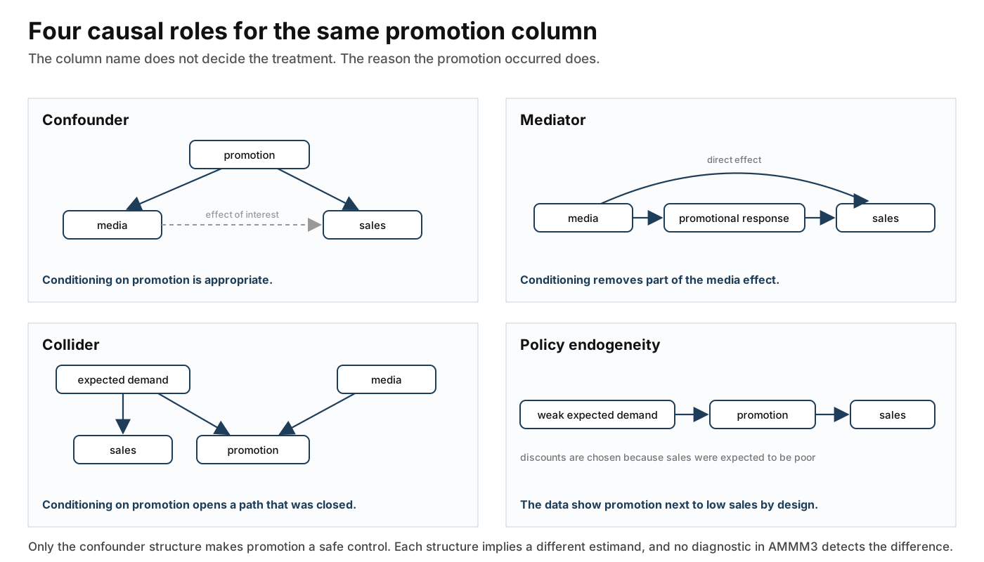
Confounder

Promotions are scheduled independently of the campaign, and they affect both media allocation and sales:

\text{promotion} \rightarrow \text{media}, \qquad \text{promotion} \rightarrow \text{sales}.

Omitting promotion confounds the media effect. Conditioning on it is appropriate. This is the case analysts assume, and it is only one of four.

Mediator

Media drives customers into a promotional funnel, or the campaign is deliberately coordinated with an offer:

\text{media} \rightarrow \text{promotional response} \rightarrow \text{sales}.

Conditioning on the downstream variable blocks part of the media effect. The media coefficient moves towards a direct effect at fixed promotional response. If the business question is “what happens to sales when we run this campaign”, removing the promotional pathway answers the wrong question, and it does so in a direction that understates media.

Branded search has the same structure, with the query volume that upstream media generates in the role of the promotional response. See Always-on and low-variance channels for how to separate that case from a channel that has too little variation to estimate.

Collider

Promotions are triggered by both weak expected demand and high planned media support, and expected demand also affects sales:

\text{expected demand} \rightarrow \text{promotion} \leftarrow \text{media}, \qquad \text{expected demand} \rightarrow \text{sales}.

Promotion is a collider on the path between media and expected demand. Conditioning on it opens a path that was closed:

\text{media} \rightarrow \text{promotion} \leftarrow \text{expected demand} \rightarrow \text{sales}.

The adjustment creates an association between media and latent demand that did not exist in the unadjusted model. This is why “add every business variable we have” is not a safe modelling principle. A collider adjustment introduces bias rather than removing it, and no diagnostic in AMMM3 will detect it.

Policy endogeneity

Managers discount because they expect products not to sell:

\text{weak expected demand} \rightarrow \text{promotion} \rightarrow \text{sales}.

The data can then show promotion coinciding with low sales, not because discounts reduce demand but because discounts are targeted at periods when sales would have been poor anyway. This is the same structure as concluding that doctors cause illness. Price and promotion share this problem: the treatment is chosen in response to the anticipated outcome. Auction-priced search spend, which rises with the demand it is meant to capture, shares it too; see Always-on and low-variance channels.

Choosing between a control and an event

Use control_columns for an ongoing covariate whose contemporaneous conditional association with the outcome is part of the specification: continuously varying market price, distribution, store count, macroeconomic indicators, weather, category demand.

Use an event surface for a discrete intervention with defined start and end dates: Black Friday, a 20% off weekend, an Easter sale, a loyalty week, a launch promotion. PanelMMM.add_events(...) and EventAdditiveEffect exist for this, with GaussianBasis, HalfGaussianBasis and AsymmetricGaussianBasis shaping the response around the date. See Additive effects and events.

The event representation has two advantages here. It states that a bounded period had an additive effect, rather than treating a campaign as a continuously measured nuisance covariate. It also does not present the promotion as an optimisable media channel.

One boundary to respect: named FE and CRE reject custom additive effects, and compute_incrementality(...) rejects mu_effects. An event-based promotion representation therefore constrains which estimators and post-fit operations remain available.

Promotional dynamics

Promotions have dynamic effects that differ in kind from media carryover. Forward buying and stockpiling move purchases earlier, so a promotion can raise sales during the offer and depress them afterwards:

\text{promotion} \rightarrow \text{purchase brought forward} \rightarrow \text{lower future sales}.

Media adstock cannot represent this. GeometricAdstock applies non-negative normalised weights to a non-negative input and feeds a saturation with positive-support beta, so the carryover is a decaying positive tail. Applying media-style adstock to a promotion imposes the wrong dynamics.

Two representations can express a sign change. AsymmetricGaussianBasis allows different widths before and after the event and an a_after amplitude that may be negative, which gives an uplift during the promotion and a dip afterwards. Alternatively, supply explicit lagged promotion columns as controls,

Y_t = \cdots + \delta_0 \text{promo}_t + \delta_1 \text{promo}_{t-1} + \delta_2 \text{promo}_{t-2} + \cdots,

where the $\delta_\ell$ are free to change sign because gamma_control is unrestricted. Construct those lags yourself; controls receive no lag transformation.

Neither representation identifies the dynamic effect. Both make it expressible, which is a precondition rather than evidence.

Optimising price is a category error

The budget optimiser solves an allocation problem over media:

\max_{\mathbf{m}} \ E[Y \mid \mathbf{m}, x] \quad \text{subject to} \quad \sum_j m_j \le B, \qquad m_j \ge 0.

Pricing is a different problem. A profit-maximising price solves

\max_p \ \pi(p) = (p - c)\, Q(p),

and the joint problem is

\max_{p, \mathbf{m}} \ (p - c)\, Q(p, \mathbf{m}) - \sum_j m_j.

The second and third require a credible demand system, cost or margin information, and usually competitor response, inventory and capacity constraints. They need stronger identification than a reduced-form sales equation supplies. AMMM3 holds none of that: the optimiser substitutes channel_data only, and its default objective is media contribution rather than profit or total outcome.

The optimiser allocates media budget. It does not solve the firm’s pricing problem. Adding price to control_columns does not change that, because the control is neither a decision variable nor part of the objective.

The deeper error is not the missing feature. It is treating a reduced-form MMM as a structural model of the firm’s whole marketing decision problem. A media MMM can reasonably estimate

E[Y \mid \text{media}, \text{price}, \text{promotion}, x].

That does not imply it has identified the potential outcome

Y(\text{media}, \text{price}, \text{promotion})

under arbitrary interventions on all three. Conditioning on a variable and intervening on it are different operations.

Worked example: when a price coefficient inverts

The example fits log units on log price as an unrestricted control. Two datasets share a true own-price elasticity of $-1.0$ and the same total variance of log price. They differ only in where that price variation comes from. In the first, price moves exogenously. In the second, 80% of the price variance comes from a latent demand signal that also raises sales, and that signal is not supplied to the model, which is the ordinary situation when demand expectations are unrecorded.

What the algebra predicts

Write the fitted specification as omitting the demand signal $d$ . Because media is generated independently of $d$ and of price, the omitted-variable result reduces to

\operatorname{plim} \hat{\gamma}_p = \gamma_p + \beta_d \frac{\operatorname{Cov}(\log P, d)}{\operatorname{Var}(\log P)}.

With $\gamma_p = -1.0$ , $\beta_d = 0.6$ , a price rule $\log P = 2.0 + 0.3 d + u$ and $u \sim \mathcal{N}(0, 0.15^2)$ :

\operatorname{Cov}(\log P, d) = 0.3, \qquad \operatorname{Var}(\log P) = 0.3^2 + 0.15^2 = 0.1125,

\operatorname{plim} \hat{\gamma}_p = -1.0 + 0.6 \times \frac{0.3}{0.1125} = +0.60.

The sign inverts when $\beta_d \gamma / \operatorname{Var}(\log P) > |\gamma_p|$ , which here means $\beta_d > 0.375$ . The inversion is not a knife-edge artefact of one parameter choice, and the bias has a ceiling of $\beta_d / \gamma$ as price becomes entirely demand-driven.

The fit

import arviz as az
import numpy as np
import pandas as pd

from abacus.mmm import GeometricAdstock, LogisticSaturation
from abacus.mmm.panel import PanelMMM

TRUE_ELASTICITY = -1.0
ENDOGENOUS_PLIM = 0.60

# Var(log price) is held at 0.1125 in both datasets. Only its source changes.
DEMAND_LOADING = 0.3
EXOGENOUS_SD = 0.15
MATCHED_SD = np.sqrt(DEMAND_LOADING**2 + EXOGENOUS_SD**2)


def make_dataset(
    price_responds_to_demand: bool, seed: int = 11, n_weeks: int = 260
) -> pd.DataFrame:
    """Return weekly log units with a known own-price elasticity of -1.0.

    ``demand_signal`` is a latent demand condition that raises sales. When
    ``price_responds_to_demand`` is True it also drives price, so the omitted
    signal biases the fitted price coefficient. Total price variance is the
    same in both datasets, so the two fits differ in bias and not in the
    amount of price variation available.
    """
    rng = np.random.default_rng(seed)
    dates = pd.date_range("2021-01-04", periods=n_weeks, freq="W-MON")
    media = rng.gamma(shape=4.0, scale=25.0, size=n_weeks)
    demand_signal = rng.normal(size=n_weeks)
    if price_responds_to_demand:
        log_price = (
            2.0
            + DEMAND_LOADING * demand_signal
            + rng.normal(scale=EXOGENOUS_SD, size=n_weeks)
        )
    else:
        log_price = 2.0 + rng.normal(scale=MATCHED_SD, size=n_weeks)
    log_units = (
        10.0
        + 0.04 * np.sqrt(media)
        + TRUE_ELASTICITY * log_price
        + 0.6 * demand_signal
        + rng.normal(scale=0.05, size=n_weeks)
    )
    return pd.DataFrame(
        {
            "date": dates,
            "media": media,
            "log_price": log_price,
            "demand_signal": demand_signal,
            "log_units": log_units,
        }
    )


def fit_price_model(dataset: pd.DataFrame, *, observe_demand: bool) -> PanelMMM:
    """Fit log units with log price as an unrestricted control.

    ``observe_demand`` adds the latent demand signal as a second control. That
    fit is only possible because this is a simulation; it is a diagnostic, not
    a remedy available on real data.
    """
    controls = ["log_price"] + (["demand_signal"] if observe_demand else [])
    X = dataset[["date", "media", *controls]]
    y = dataset["log_units"]
    mmm = PanelMMM(
        date_column="date",
        target_column="log_units",
        channel_columns=["media"],
        control_columns=controls,
        control_impacts=dict.fromkeys(controls, "unrestricted"),
        adstock=GeometricAdstock(l_max=4),
        saturation=LogisticSaturation(),
    )
    mmm.fit(
        X,
        y,
        draws=500,
        tune=500,
        chains=2,
        cores=2,
        progressbar=False,
        random_seed=42,
    )
    return mmm


def implied_elasticity(mmm: PanelMMM) -> tuple[float, float, float]:
    """Return the posterior mean and 94% HDI of the implied price elasticity.

    ``gamma_control`` is estimated against the scaled target, so it is
    multiplied by the target scale to return to log-units.
    """
    gamma = mmm.idata.posterior["gamma_control"].sel(control="log_price")
    elasticity = gamma * float(mmm.data.get_target_scale())
    hdi = az.hdi(elasticity, hdi_prob=0.94)["gamma_control"].values
    return float(elasticity.mean()), float(hdi[0]), float(hdi[1])


exogenous = make_dataset(price_responds_to_demand=False)
endogenous = make_dataset(price_responds_to_demand=True)

results = {
    "exogenous price": implied_elasticity(
        fit_price_model(exogenous, observe_demand=False)
    ),
    "price set from demand": implied_elasticity(
        fit_price_model(endogenous, observe_demand=False)
    ),
    "price set from demand, signal observed": implied_elasticity(
        fit_price_model(endogenous, observe_demand=True)
    ),
}

print(f"true elasticity                          {TRUE_ELASTICITY:+.2f}")
print(f"predicted limit when price is endogenous {ENDOGENOUS_PLIM:+.2f}")
for label, (mean, lower, upper) in results.items():
    print(f"{label:40s} {mean:+.2f}  [{lower:+.2f}, {upper:+.2f}]")

That prints:

true elasticity                          -1.00
predicted limit when price is endogenous +0.60
exogenous price                          -0.95  [-1.14, -0.76]
price set from demand                    +0.55  [+0.46, +0.64]
price set from demand, signal observed   -1.00  [-1.03, -0.97]

Three fits, three outcomes. With exogenous price variation the posterior recovers $-0.95$ , covering the true value. With price set from omitted demand the posterior sits at $+0.55$ , near the predicted limit of $+0.60$ and confidently on the wrong side of zero: the model says raising price sells more units, and its 94% interval excludes both zero and the truth. Adding the demand signal to the same endogenous dataset returns the estimate to $-1.00$ , which shows the failure is the omission and not the estimator, the priors or the sampler.

Note the interval widths. The endogenous fit is the most precise of the three wrong answers, because the demand signal it absorbs is a strong predictor. A narrow posterior on a biased coefficient is the expected outcome here, not a warning sign.

Two implementation details. The target is supplied already logged, because target_type is reporting metadata and does not change the fitted functional form. gamma_control is estimated against the scaled target, so recovering an elasticity requires multiplying by the target scale from mmm.data.get_target_scale().

What this demonstrates and what it does not

It demonstrates four things. The same specification returns a usable elasticity or an inverted one depending only on how price was set. Nothing in the fit distinguishes the two cases, because convergence diagnostics and predictive checks are satisfied in both. The posterior interval in the endogenous fit is narrow and excludes the true value, so precision is not evidence of correctness. The third fit identifies the cause as the omitted driver.

It does not offer a correction you can apply. The third fit uses a column that exists only because the data were simulated. On real data the demand signal is whatever management knew and did not record, and a partial proxy reduces the bias without removing it. It also does not show that any particular real price coefficient is biased, only that the fit cannot tell you.

A directional prior does not help here. Constraining the price coefficient to be negative would move the posterior off $+0.55$ without recovering the true $-1.0$ , producing a plausible-looking negative interval that reflects the constraint rather than the data. That is worse than the visible inversion, because the inversion is at least detectable.

Before adding price or promotion

Price and promotion are not automatically controls. Adding a variable to control_columns conditions the outcome model on that variable. It does not establish that the variable is exogenous, give it carryover or saturation, or make it available to the budget optimiser.

Price and promotion are frequently chosen in response to expected demand and may therefore be endogenous. Promotion may additionally be a mediator or a collider in the media to sales relationship. Conditioning on such variables can change the estimand or introduce bias.

Work through these in order.

State the estimand. Total media effect, media effect at fixed price and promotion, price elasticity, or conditional prediction.
Draw the causal role of each variable. Confounder, mediator, collider, or simultaneously determined. Record the reasoning.
Decide the functional form. Log price, relative price, or deviation from a reference price, and whether asymmetry matters.
Choose the representation. Control column, lagged control columns, or an event surface, and check the estimator and operation contracts that choice implies.
Report the coefficient within its claim class. Do not promote a control coefficient to an elasticity without an identification argument.

Reporting language

Conditional model result. “In a model of log revenue conditioning on log price, media and seasonality, the log-price coefficient has a posterior mean of X. This is a conditional association. Our pricing process responds to expected demand, so we do not report it as an own-price elasticity.”

Narrower estimand. “Conditioning on promotional activity, the media coefficient estimates the media effect at fixed promotional response. It is not the total effect of running the campaign, because the campaign also changes promotional response.”

Declining the request. “Price is not a decision variable in this model. The optimiser allocates media budget against media contribution, and it holds no margin or cost information, so it cannot evaluate a pricing decision. A pricing recommendation needs a demand model with an identification strategy and margin data.”

Causal evidence. “In a randomised price test across matched stores over eight weeks, a 5% reduction raised unit sales by Y% with a stated interval. That estimate applies to that range, period and set of stores.”

Do not describe a control coefficient as an elasticity. Do not present a promotion coefficient as the return on promotional investment when promotions are scheduled in response to expected demand. Do not report a media coefficient estimated with a promotion control as the total effect of the campaign.