Interpreting Optimisation

After you run budget optimisation, you usually work with three outputs:

the allocation DataArray
the SciPy OptimizeResult
a simulated response dataset from sample_response_distribution()

This page explains how to read each one.

Read the optimiser output

PanelBudgetOptimizerWrapper.optimize_budget(...) returns:

allocation, result = wrapper.optimize_budget(...)

If you set callback=True, it returns a third value:

allocation, result, callback_info = wrapper.optimize_budget(..., callback=True)

`allocation`

allocation is an xarray.DataArray over the non-date budget dimensions.

Model shape	Typical allocation dims	Meaning
No extra panel dims	`("channel",)`	One optimised value per channel
`dims=("geo",)`	`("geo", "channel")`	One value per `(geo, channel)` cell
`dims=("geo", "brand")`	`("geo", "brand", "channel")`	One value per `(geo, brand, channel)` cell

The values are in the wrapper’s per-period units. Unoptimised cells are present and set to zero.

`result`

result is SciPy’s OptimizeResult. The fields you will usually inspect are:

Field	Meaning
`success`	Whether the solver converged
`status`	SciPy status code
`message`	Human-readable solver message
`fun`	Final objective value
`nit`	Number of iterations
`x`	The optimised flat parameter vector

If success is False, AMMM3 raises MinimizeException unless you opt in to return_if_fail=True on the underlying BudgetOptimizer.

`callback_info`

When callback=True, AMMM3 records one entry per solver iteration. Each entry includes:

x
fun
jac
constraint_info when constraints are active

Use this when you need to diagnose solver behaviour rather than just consume the final allocation.

Simulate the optimised plan

The optimiser itself returns only the allocation. To estimate spend paths and contributions over the requested window, call sample_response_distribution().

response_samples = wrapper.sample_response_distribution(
    allocation_strategy=allocation,
    noise_level=0.0,
    include_last_observations=False,
    include_carryover=True,
    budget_distribution_over_period=budget_distribution,
)

Set noise_level=0.0 when you want the spend path to match the requested allocation exactly.

What `response_samples` contains

The wrapper builds a synthetic future dataset, samples posterior predictive draws, and then merges the requested allocation and simulated spend path back into the result.

response_samples therefore contains:

Variable	Source	Meaning
`allocation`	Added by the wrapper	Requested allocation without a `date` dimension
One variable per channel	Added by the wrapper	Simulated spend path over the future dates
`mmm.output_var`	Posterior predictive sample	Model output variable
`channel_contribution`	Posterior predictive sample	Channel contribution on model scale
`total_media_contribution_original_scale`	Posterior predictive sample	Total media contribution on the original target scale

If you pass additional_var_names, AMMM3 also includes those variables when they exist in the model graph.

Carryover and evaluation window

include_carryover=True changes how AMMM3 builds the synthetic future window.

AMMM3 extends the generated dates by adstock.l_max periods.
It then zeroes the tail spend rows after the requested window.
The extra dates let posterior predictive sampling include lagged effects from the planned spend.

This is why the simulated dataset can cover a longer evaluated window than the requested start_date to end_date range, while still preserving the same total spend.

Plot the result

The plotting helpers under mmm.plot are designed to work directly with the response dataset returned by the wrapper.

fig, ax = mmm.plot.budget_allocation(response_samples, original_scale=True)

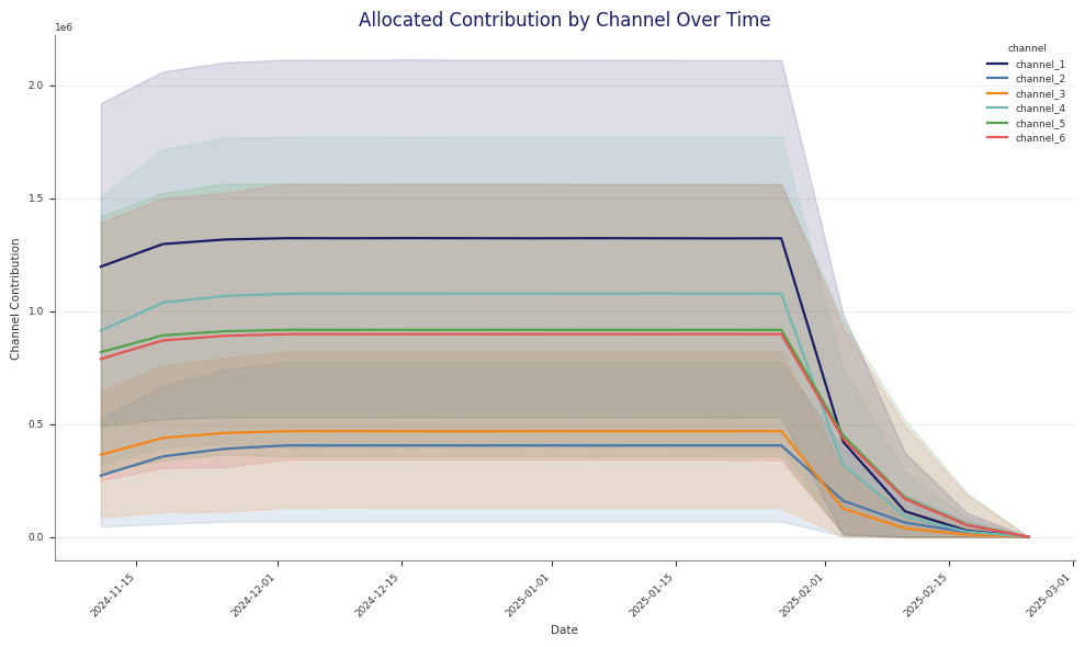
fig, ax = mmm.plot.allocated_contribution_by_channel_over_time(
    response_samples,
    original_scale=True,
)

Useful options:

dims={...} to filter a panel slice
split_by="geo" or another dimension to create separate subplots
original_scale=True to prefer original-scale contribution variables when they are available

Example optimisation output:

Budget allocation example

Allocated contribution by channel over time

Budget response curves example

Read the Stage 70 pipeline artefacts

If you run optimisation through python -m abacus.pipeline.runner, Stage 70 writes both the low-level optimiser output and several interpretation files.

File	What it contains
`optimized_allocation.nc` / `optimized_allocation.csv`	The allocation returned by the optimiser
`response_distribution.nc`	The simulated response dataset for that allocation
`optimize_result.json`	Solver status, message, objective value, and iteration count
`budget_summary.csv`	Current versus optimised totals
`budget_response_points.csv`	Per-channel current versus optimised spend, contribution, and efficiency summaries
`budget_impact.csv`	Delta between current and optimised channel summaries
`budget_bounds_audit.csv`	Current spend, scaled reference spend, bounds, optimised spend, and bound checks
`budget_roi_cpa.csv`	Channel efficiency summaries using the model’s efficiency metric
`budget_response_curves.csv`	Saturation-only response curve summaries
`budget_mroi.csv`	Marginal efficiency estimates at the current and optimised spend points

The stage also writes plots for allocation, contribution over time, response curves, impact, bounds audit, and ROI or CPA summaries.

These Stage 70 spend figures are reported in total horizon spend units so they can be compared directly to current historical spend over the same reference window. AMMM3 still converts to the low-level wrapper’s per-period budget contract internally.

Practical checks

Before you use an optimised plan, check:

result.success and result.message
whether the allocation matches your intended budget units
whether budget_bounds_audit.csv or your own checks show any bound issues
how much of the gain comes from reallocation versus carryover assumptions
whether the point lies on a sensible part of the response curve, not just on the edge of a bound

For multi-plan comparison in total horizon units, use Scenario Planning.